Live analyzing movement through machine learning
This post was originally published on Engineering@TelenorDigital.
Twice a year Telenor Digital organises an internal hackathon, a two-day offsite where we have the chance to mingle with other teams and work on things we’d normally never touch. Given Jan’s fascination with phone sensors he was wondering whether we could feed the data from the gyroscope and the accelerometer into a machine learning algorithm and that way classify what a person is doing. Could we create a model that would check the stream of data coming off these sensors and then tell whether the person is sitting, walking or dancing?
We quickly assembled our dream team consisting of Bjørn Remseth, who took a class or two in machine learning; Audun Torp, a mathematician; and Jan Jongboom, a certified data gatherer. And with that we were off to work, having 36 hours to start building our classifier…
Gathering data
The first step in training a model is to acquire some test data. In this phase there’s no fancy processing, but just recording data of the sensors, tagging it with a movement (sitting, walking, dancing) and storing it. To get up to speed as fast as possible we decided to hack together a simple JavaScript web application that uses the device orientation and device motion APIs to acquire data from the gyroscope (alpha, beta, gamma axes) and the accelerometer (x, y, z axes); giving us six data streams to work with.
The web application is connected over a web socket to a node.js server sitting on a laptop, and creates per measurement a CSV file that contains the timestamp and the raw data from each of the sensor axes. The application we built is hosted on GitHub, and outputs it’s data into the ‘raw-data’ folder.
To get some nice training data, we then take an ordinary Android or iOS phone, navigate the browser to the client web page, and hit ‘Start measurement’. For 30 seconds (indicated by beeps every 10 seconds) we then record the data, and later tag it by renaming the file to something like ‘jan-dancing-v1.csv’.
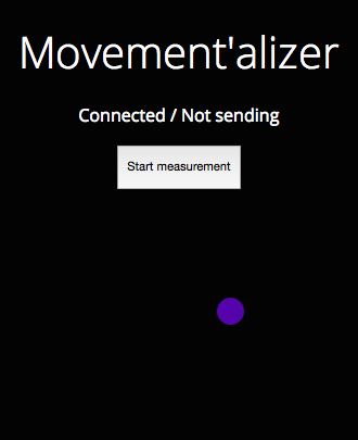
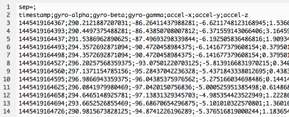
Data gets measured 30 times per second and dumped into a file
Just plotting the gyro data into Excel already gives us some interesting insights. We see the steps happening on ‘gyro-beta’ (upper leg moving front to back), and we see me turning around at the end of the room at ‘gyro-alpha’. Now humans are great at pattern recognition, but can we train a computer to do the same?
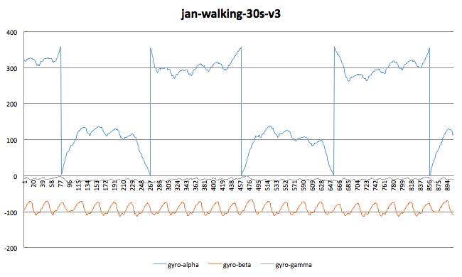
The vertical lines are an artifact coming from the fact that we use a 0-360 degree scale that wraps around
Training the model
The problem we are solving is a classification problem: Given some data, we must determine which label in a list of labels best describes the data.
Bjørn’s summary of the machine learning courses he has taken is that machine learning is very glamorous and all, but here are also a list of dirty secrets that one have to keep in mind: The first is that any almost halfway decent algorithm can give results that are useful if they are given a proper learning set (the classical on this issue is Brillo and Bank’s paper from 2001, which shows that for small training sets there is great difference between algorithm performance, for large datasets the difference is much less). The second is that there are a bunch of different algorithms, and they all have their own peculiarities that it can easily take months to get a grip on. The third is that it’a very easy to get lost in all of this variation.
So based on this our overall plan was:
- Start right away sampling data and get as much as we could of it as soon as possible.
- Select a framework to work within. We ended up selecting scikit-learn, simply because it turned up on top of a google search and a quick inspection of the examples indicated that it wold be an OK choice (it was).
- Read some example code and hack up something that worked immediately. The example code used a support vector machine classifier, and that choice we stuck to for the duration of the hackathon.
filters = {'dancing': 0, 'walking': 1, 'sitting':2}
if arguments['--model']:
    clf = joblib.load(arguments['--model'])
else:
    training = dataset('../datasets/training', filters)

    svr = svm.SVC()
    exponential_range = [pow(10, i) for i in range(-4, 1)]
    parameters = {'kernel':['linear', 'rbf'], 'C':exponential_range, 'gamma':exponential_range}
    clf = grid_search.GridSearchCV(svr, parameters, n_jobs=8, verbose=True)
    clf.fit(training.data, training.target)
joblib.dump(clf, '../models/1s_6sps.pkl')- Find some way to track progress. We ended up using scikit-learn’s built-in precision/recall calculation for that, and tracked the progress over time in a csv file.
All of this was accomplished rather quickly, so we figured we could spend the rest of the time figuring out how to make the model better. Unfortunately that took a lot of time and did not give us much progress.
Simplifying the problem
To get going we made some simplifications:
- We only looked at the beta-channel from the gyros, which measures front-back tilt. We figured that we could integrate more data later.
slice = self.data[first:last]
slice = [column[1] for column in slice]
Column [1] is the beta channel of the gyroscope, and that is the only
thing we care about when we do feature extraction and analysis.
- We chopped the data into three second segments, and then performed a discrete fourier transform (using the fast fourier transform “FFT”), chunking into buckets and removing all components with higher frequencies than 5 Hz (by inspection it didn’t seem to be much of interest in higher frequency parts of the spectrum anyway). These truncated and chunked FFT spectra were then used as feature vectors by the machine learning algorithm.
The feature vectors are simply FFT power spectra:
transformed = fft.fft(slice)
absolute = [abs(complex) for complex in transformed]

frequencies = self.get_frequencies()

buckets = [0 for i in range(num_buckets)]
width = hertz_cutoff / num_buckets
sum_of_buckets = 0.0000001
for i in range(1, len(absolute)):
    index = int(frequencies[i] / width)
    if index >= num_buckets:
        break;
    buckets[index] += absolute[i]
    sum_of_buckets += absolute[i]

if arguments['--normalize']:
    buckets = map(lambda x: x/sum_of_buckets, buckets)
The 0.0000001 is just to avoid dividing by zero when normalizing, if the data consists of only zeros, it’s a hack, it’s a hackathon, these things happen …
The parameters that we’re passing into this function are the number of bucket’s we’re using (40) and the cutoff frequence (5 Hz), giving the buckets a resolution of 1/8 Hz.
It turned out that these two adaptations were the only two that we could prove actually made sense. We made a plot of the time evolution of the precision/recall performance of our classifier:
# Write precision/recall to a file so that we can se how
# the precision of the project's output improves over time.
ts = time.time()
record = str(ts) + ", " +  str(precision) + ", " +  str(recall) + "\n";
with open("../logs/precision-recall-time-evolution.csv", "a") as myfile:
    myfile.write(record)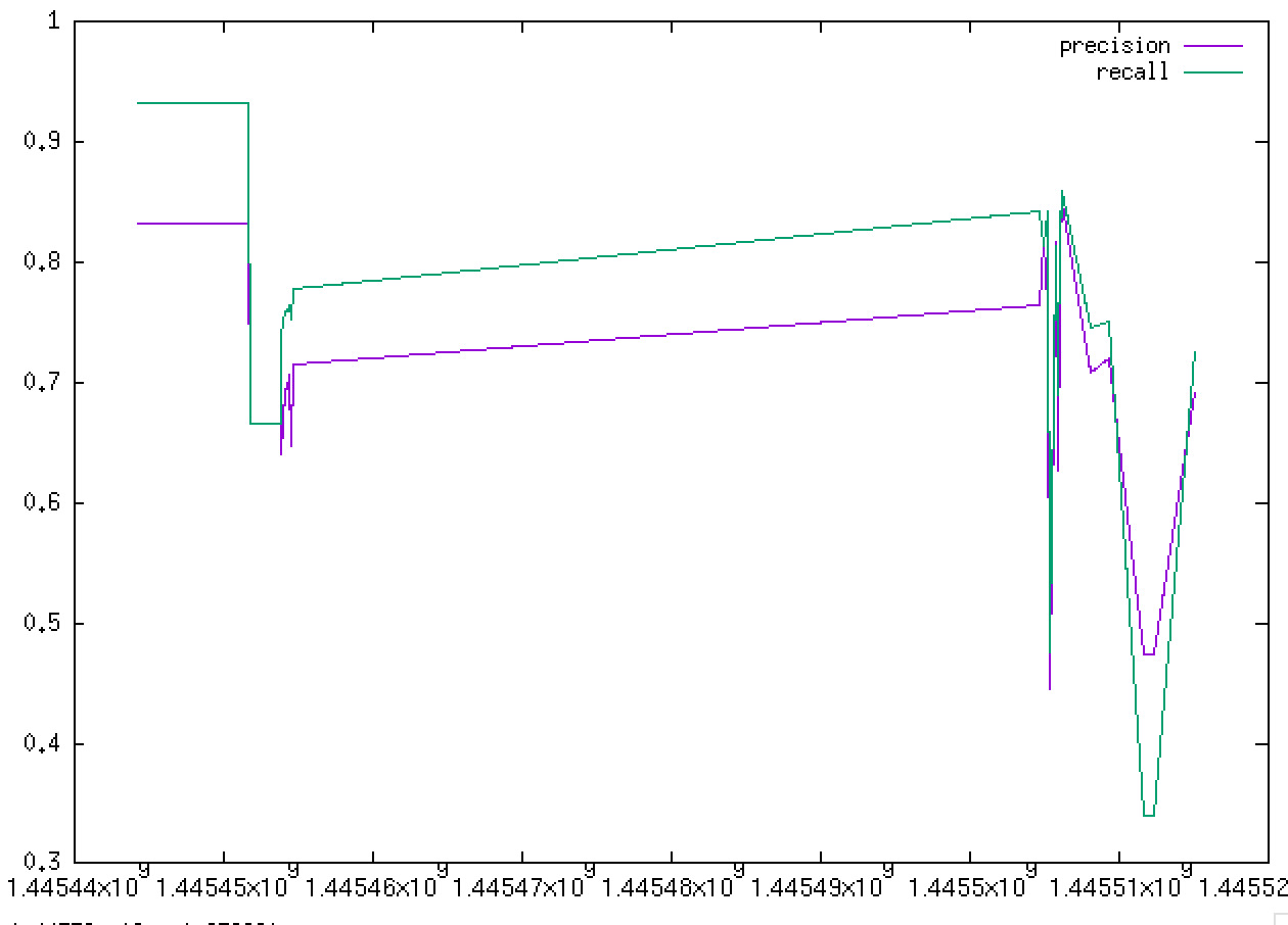
The x-axis is time in seconds since epoch (because, unix). The plot starts right after we got the first data in, and we ran it through the classifier and found that it was amazingly good. Unfortunately we were looking at 30 second samples, not three second samples so we were in all likelihood overfitting. When we chopped things into 3 seconds samples performance got a lot worse. Then it improved a little as we removed some trivial bugs. Then we went home to sleep (which shows up as the straight line in the plot).
Improving the model
When we got to work the day after, we had a long list of clever tricks we wanted to use: Integrate more data into the feature vectors; dimensionality reduction using principal component analysis (PCA) before doing FFT along the dataset projected along the primary principal component (the one along the axis of maximum variation); and proper normalisation of the FFT spectra (so that they all sum to one). We tried these, and they consistently gave us worse results than the initial scheme. The one thing that gave somewhat better results were to look at differences between samples instead of the samples themselves before taking FFT of them.
We are pretty certain that the classifier we produced can be improved a lot: It only uses one channel out of six; it doesn’t use any of the fancy techniques that are supposed to tease information out of multidimensional datasets (e.g. PCA); it doesn’t use know best practices (e.g. normalisation of feature vectors); and it still uses the SVM classifier for no other reason that being the first (and only) one we tried. Most likely there are other classifiers that work as well or better than that. Given all this, we’re certain that this result can be improved significantly. However, there are at least two really good things to be said about our classifier:
- It actually works.
- We have the numbers (and a graph) that indicates how well it works so
if/when a better way is found, it will be evident that it has been found.
Live classifying the data
Now that we have a trained model we can start classifying data as it flows in. For this we can re-use the app we used for data gathering. As it already writes to a file whenever new data flows in we can have our Python application monitor the directory and read the last touched file. Then take the last 3 seconds and feed it into the classifier (cleaned up a bit for readability):
data_feed = arguments['--data']

if data_feed:
    print "Monitoring folder " + data_feed
    while True:
        try:
            all_files_in_df = map(lambda f: os.path.join(data_feed, f), os.listdir(data_feed))
            data_file = max(all_files_in_df, key = os.path.getmtime)

            sample = sample_file(data_file)
            # get 6 seconds * 30 samples
            sample.keep_last_lines(180)
            samples = sample.get_samples()

            # dump the classification into a file
            pr = clf.predict(samples)
            with open('../data-gathering/classification', 'w') as f:
                f.truncate()
                f.write(str(pr))
        except:
            print "Unexpected error", sys.exc_info()[0]

        time.sleep(1)
This reads data from the data-gathering application, and writes the result from the classifier back to a file, looking something like this, where the numbers on the right are the most recent:
[0 2 2 2 0 0 0 1 1 0 1 0 0 0 0 0 2 2 2 2 2 2 2 2 2 2 2 2 2 2]
0=sitting, 1=walking, 2=dancing
In the node.js app we can monitor the classification file, and then send this data over a web socket to a web browser to visualise the movement:
fs.watch('./classification', function(curr, prev) {
  fs.readFile('./classification', 'utf-8', function(err, data) {
    if (err) {
      return console.error('Cannot read classification file', err);
    }
    broadcast(JSON.stringify({
      type: 'classification',
      classification: data.match(/\d/g)
    }));
  });
});
Based on that we can create a simple web page that then shows this data to the user, giving live feedback on what the classifier thinks he’s doing at this very moment!
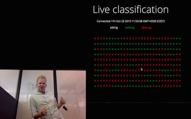
The classifier giving live feedback on the computer screen on what the model thinks Jan is doing. This is all based on just one axis of his phone’s gyroscope in his front pocket.
Conclusion
We were incredibly surprised how far we managed to get in 36 hours. The classifier is rough around the edges, and more training data probably helps, it’s surprising to see how well the classifier already manages to distinguish movement. It’s even more surprising to see that we even managed to get proper results by just using one out of the six axes. Just imagine how much better this can get with more data. Machine learning is really maturing.
I’d like to encourage everyone reading this to actually try our project. We already trained the model, and all code and instructions are listed in this GitHub repo. You’ll just need a phone. Of course you can just throw away our model and use our code to train a completely new one. To get you started we already included some data of people walking up the stairs. Try feeding that data into the model, and see what happens. We’d love to see your results!